Whether you are a broker, CFO, or risk manager, you have probably heard the terms loss development triangle, loss development factor, and IBNR (incurred but not reported losses). These are often included in the first analytical step of an actuarial analysis. Yet a survey of insurance professionals would likely result in a long list of contradictory definitions for these terms. Because of the importance of this topic and the confusion it causes, we have selected it for an in-depth blog article.

Loss development is one of the most challenging actuarial topics for non-actuaries.  For those familiar with the topic, this article will be a good review and perhaps provide some new insight. For those unfamiliar with loss development or any of the terms mentioned above, don’t worry. We will walk through an example, explain every term, and unlock the “black box” of loss development factors, loss triangles, and even IBNR.

Loss Development: Some Old Claims Never Die, They Just Get Adjusted
It may take several years for all claims in a given policy period to be reported and closed. New information pertaining to existing claims can impact the total losses long after the end of a policy period. Unfortunately, even new claims are sometimes reported after the close of the policy period. Therefore, a snapshot, or summarized evaluation of the losses, is generally made at least once a year. The development in the losses is the quantitative change in this evaluation from year to year.

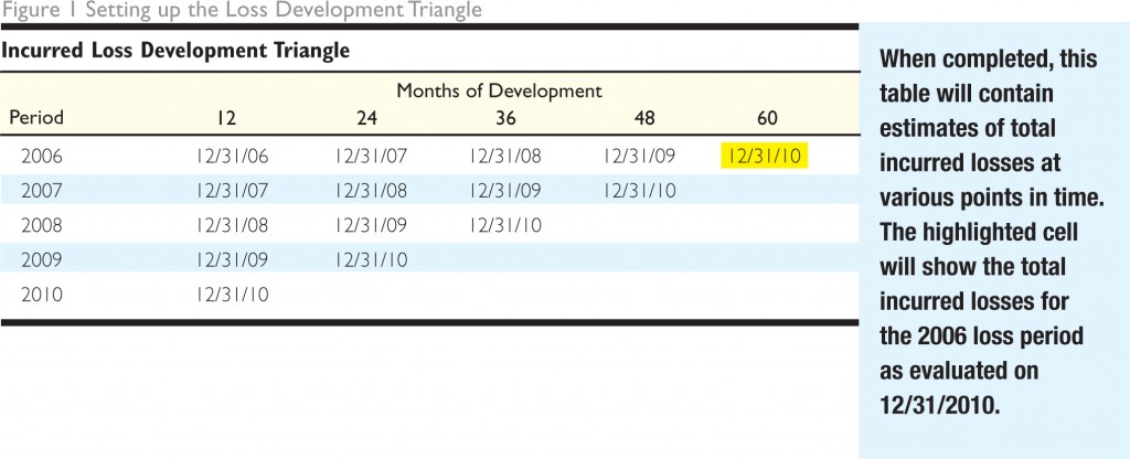
A loss development triangle is a unique way of arranging the annual loss evaluations for several past policy periods. By arranging the loss evaluations for past years in a table, we can analyze the change in losses from one evaluation to the next. The standard format is shown below. Note how the evaluations are aligned in columns according to the length of time since the inception of the policy period.

The purpose of arranging data this way is to estimate the development, or change in estimated losses, from one evaluation to the next. The table should include as many years of historical data as is available. There are two primary reasons that development occurs:

• Sometimes losses that occur during a certain period are not reported until a later date. These additional loss dollars are referred to as incurred but not reported losses. A common abbreviation for this term is IBNR.
• Case reserves, amounts set aside for future payments on a claim, must sometimes be adjusted as more information about a loss becomes available. Adjustments are also made to claims that have been closed and reopened. For example, a back injury that occurred a few years ago may have been established with a $50,000 reserve, but later data shows that the actual costs have reached $80,000 and are anticipated to grow to $100,000 due to ongoing treatments related to the original injury. This “growth” in the claim results in loss development.

When you look at several years of data and snapshots of the loss reserves, you begin to see a trend. Once development between evaluations has been estimated, the total anticipated development can be computed for any evaluation date. An example is provided later in this article.

The Required Data
Data is usually gathered on both paid and reported losses. Paid losses are the total losses actually paid during a policy period. Reported losses (also referred to as incurred losses) include paid losses plus any loss reserves for open claims. Reported losses are always greater than or equal to paid losses. There are pros and cons as to which type of data is more useful when generating a loss triangle:

• A reported loss triangle is most useful when the claim reporting pattern and reserving philosophy are consistent for each loss period. Development patterns based on reported losses tend to be less volatile than patterns based on paid losses. This is because the initial reported amount of a claim, as compared to the initial paid amount, is usually closer in value to the ultimate amount. Therefore, the reported loss amount varies less than the paid amount over time.
• A paid loss triangle is most useful when the claim payment pattern and claim settlement philosophy are consistent for each loss period. In addition, since case reserves are excluded, development patterns are not skewed by changes in reserving philosophies.

If both paid and reported loss information is available, it is common to create a loss triangle using both methods and then decide which method produces the most reliable results. This decision is based primarily on the volatility of the development patterns. The data should be segregated between lines of coverage such as auto, general liability, workers compensation and others. The data can be limited to a certain per occurrence loss limit, but only if all claims for all periods are limited to the same value. For example, you may want to use limited losses if you are projecting losses within a certain range, like under $100,000. This might occur if an insurance program is being considered with a $100,000 deductible. There may be other reasons why you might want to forecast losses under a specific loss limit.

The number of loss periods you will need to create a credible analysis varies based on a number of factors. Five to ten years of data is often sufficient. You will also need industry development factors as a standard to measure against. These are available through various data-gathering organizations such as the National Council on Compensation Insurance (NCCI) and the Insurance Services Office (ISO), publications such as Best’s Aggregates & Averages, and brokers, actuaries and insurance companies.

Completing the Loss Triangle and Selecting Factors
In most cases, losses increase from one evaluation to the next. Once we have our data gathered and the loss information entered into the loss triangle, the next step is to measure the increase.

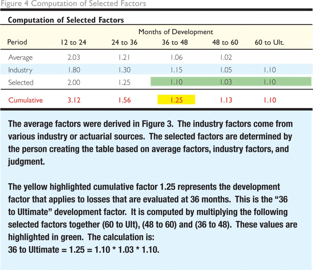
After we complete the table shown in Figure 2, we are ready to compute the development between each evaluation. In the footer of Figure 3, averages of the factors are computed. The average is the straight average of each column. When the data is more volatile, other averages such as a weighted average, two or three-year averages, or an average that excludes the high and low points could be used. These average values are carried forward to Figure 4 along with industry factors.

Selected factors are usually a combination of the unique averages and industry factors.  Additional information concerning the losses, changes in reserve practices, implementation of loss control or prevention programs, or other considerations may also influence the determination of the selected factors. Careful consideration of such subjective data is where actuarial judgment, beyond simply following a formula, enters the process of selecting factors.

Using the Results
We now have a completed loss development triangle and selected loss development factors. The next step is to apply the information. The ultimate incurred losses for each loss period can now be estimated. For example, the 2010 12-month evaluation of $1,225,750 is multiplied by the 12-month-to-ultimate loss development factor of 3.12 to yield an estimated ultimate loss amount of $3,824,340. See Figure 5 below.

The development factors applied to incurred losses are selected based on the time that has passed between the beginning of a loss period and the evaluation date of the loss. In most cases, the closer the evaluation date is to the period effective date, the larger the loss development factor will be. This reflects the significant amount of unknown factors that may affect relatively new claims. Conversely, as the period matures the loss development factors approaches 1.00. Loss development factors are a key component of an actuarial analysis. Developing unique factors based on historical data provides for more accurate estimates. Understanding loss development factors lays the foundation for a more in-depth explanation of IBNR, which will be explored in a future article.

We welcome your feedback by posting a comment or contact us at support@SIGMAactuary.com.

Don’t forget to register for our free resource portal by visiting https://www.sigmaactuary.com/education/
© 2011 SIGMA Actuarial Consulting Group, Inc.